12 Regression with Qualitative Independent Variables
In this chapter, I will walk you through some analysis I conduct with an example dataset, in order to show how regression works with qualitative independent variables. I could have easily completed this analysis using the methods from Chapter 8, but it is important to see how regression can also be used as a method for comparing means across groups.
Let’s say I’m interested in studying how personality relates to sex. The most common model of personality in psychology is called the “Big Five.” One common measure consists of 50 survey items (the IPIP Big-Five Factor Markers), with 10 items for each of the five personality traits from the model.1 Figure 12.1 shows some of these questions and how they are formatted.
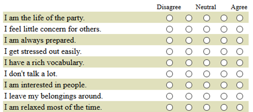
For now, I decide to focus on whether people are introverted or extroverted. Extroverts are outgoing and tend to enjoy interacting with others. Extroverts will tend to agree with the statement “I am the life of the party” while introverts will tend to agree with the item “I don’t talk a lot.”
I find a dataset that contains lots of responses to the Big Five personality questions as well as information on the sex of each respondent.2 There are 10 different questions related to extroversion, and the dataset has one variable for each of these 10 questions (Figure 12.2). The variable labeled e1 shows responses to the item “I am the life of the party.” A value of 1 means the respondent disagrees with this statement, while a 3 indicates neutral, and a 5 means they agree.
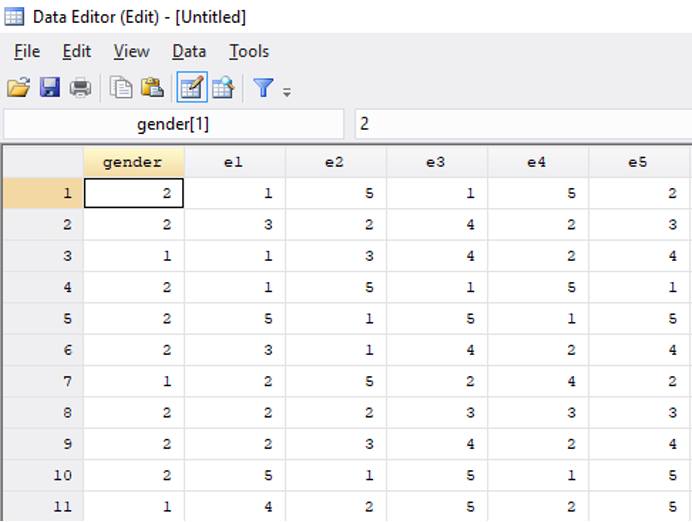
For all of the odd-numbered extroversion questions (e1, e3, e5, etc.), agreement indicates extroversion. For the even-numbered items (e2, e4, e6, etc.), agreement indicates introversion. To create a single extroversion variable that combines responses from all 10 survey items, I create a tally, adding up all the values for odd-numbered questions and then subtracting the responses to the even-numbered questions. An extreme extrovert will have a 5 for all the odd-numbered questions and a 1 for all of the even-numbered ones, giving them a score of 20 (\(5 \times 5-5 \times 1=20\)). An extreme introvert will have a -20 since they will answer 1 to all the odd-numbered questions and 5 to all the even-numbered ones (\(5 \times 1-5 \times 5=-20\)).
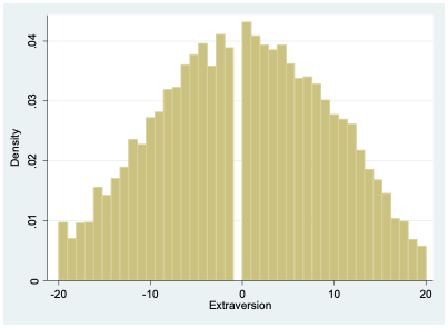
As Figure 12.3 indicates, most people lie somewhere in the middle between introversion and extroversion.
Our sex variable was measured by asking respondents “What is your gender?” Selection of male was coded as a 1, while selection of female was coded as a 2.
12.1 Predicting extroversion using sex
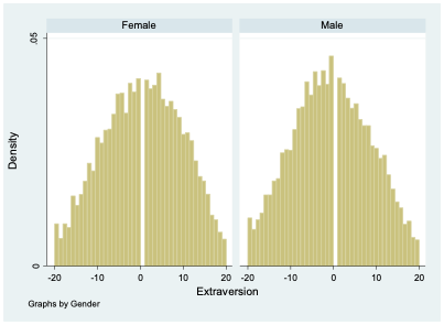
If I want to describe differences in extroversion by sex in this dataset, I can compute the mean value of extroversion for males and for females. It turns out that males have an average extroversion of -0.46 while females’ average level of extroversion is 0.53. Thus, the average female is about 1-point more extroverted than the average male. But of course, there is abundant variation in extroversion among both groups, as seen clearly in Figure 12.4. There are plenty of females who are introverts and plenty of males who are extroverts.
If you asked me to guess the extroversion level of someone in this dataset and the only thing you told me about them was their sex, my best bet would probably be to guess the average extroversion level for someone of that sex. So for a female I knew nothing else about, I would guess their extroversion to be 0.53, while for a male I’d guess -0.46.
When we’re working with data, sometimes it’s helpful to express how I would make a guess about a dependent variable (extroversion) based on an independent variable (sex) using a mathematical formula. In fact, this is exactly what we do when we run a regression. There are many ways I could write this formula, but I’ll show just two for now. First, I could write:
\[ \widehat{Extraversion}=0.53 \times Female-0.46 \times Male \tag{12.1}\]
Notice I’ve added a “hat” above the name of the variable Extraversion; this hat means that I’m making a guess about the value of that variable (I’m guessing the level of extroversion based on sex). The equation has two other variables Female and Male, and these two variables will take on a value of 1 if the person’s sex is equal to the name of the variable and will otherwise take on a value of 0. For a female, Female will equal 1 and Male will equal 0, giving us:
\[ \widehat{Extraversion}=0.53 \times (1)-0.46 \times (0)=0.53 \]
So our guess for the level of extroversion (\(\widehat{Extraversion}\)) of a female we know nothing about is 0.53.
For a male, our guess is:
\[ \widehat{Extraversion}=0.53 \times (0)-0.46 \times (1)=-0.46 \]
There’s a second way I can write my formula, which will turn out to be more useful in the future when we come to consider multiple factors at the same time that might help us predict the value of a dependent variable. Rather than having two variables to represent sex in my equation, I can just use one:
\[ \widehat{Extraversion}=0.53-0.99 \times Male \tag{12.2}\]
In Equation 12.2, we start from female as our baseline. Notice that the first number we see (0.53) is our guess for the value of extroversion for a female. When we’re considering a female, Male=0, so:
\[ \widehat{Extraversion}=0.53-0.99 \times 0=0.53 \]
Thus, we get the right prediction for females from this equation, even though we didn’t include a variable specifically for females. If we have a male, Male=1, so we get:
\[ \widehat{Extraversion}=0.53-0.99 \times 1=-0.46 \]
This is the same prediction we got before. Remember, I decided to initially just analyze respondents who selected either male or female. Since we are only considering two categories (male or female), and each respondent is either a male or a female, saying Male = 1 lets me know that Female = 0. It’s actually repetitive in this context to both say that Male = 1 and Female = 0. Similarly, saying Male = 0 implies that Female = 1. So I can simplify my equation by just including one variable to indicate binary sex.
Notice that in Equation 12.2, the number next to Male is equal to the difference between the average level of extroversion for females and the average level for males (0.53-(-0.46)=0.99). This is because Equation 12.2 starts with females as the baseline, so to get our prediction for males, we have to adjust our baseline prediction by the average difference for males.
Equation 12.2 is also typically how we will arrange our equation when we’re running a regression.
Goldberg, L. R. (1992). The development of markers for the Big-Five factor structure. Psychological assessment, 4(1), 26.↩︎
https://openpsychometrics.org/_rawdata/ (the file I used is called “BIG5.zip”)↩︎